07. 手动调整参数

调整参数

似乎上次的 3 个算法当中,有 2 个效果不错,对吧?以下是你可能会获得的图形:
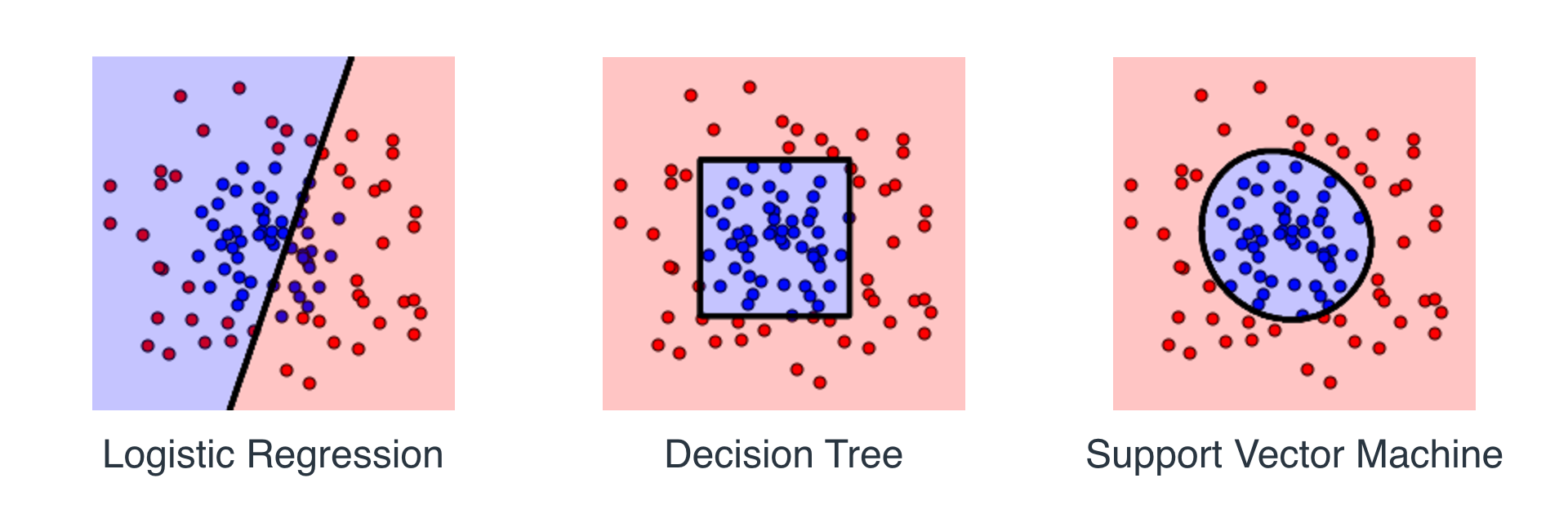
似乎逻辑回归的效果不太理想,因为它是线性算法。决策树能够很好地划分数据(问题:决策树的界限区域为何是那样的?),SVM 的效果非常棒。现在我们试试稍微复杂些的数据集,如下所示:
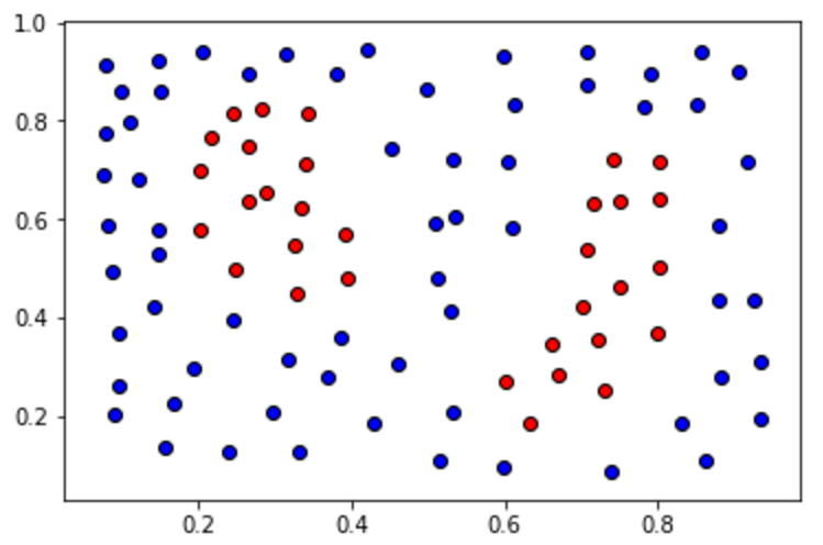
我们试着用 SVM 分类器拟合此数据,如下所示:

 classifier = SVC()
 classifier.fit(X,y)

如果输入上述内容,将失败(你将有机会在下面试试)。但是,也许我们没有充分利用 SVM 分类器。首先,我们使用了正确的内核吗?例如,我们可以使用 2 次多项式内容,如下所示:

classifier = SVC(kernel = 'poly', degree = 2)

我们自己试试,看看这些参数。稍后我们将深入了解这些参数,但是你可以设定以下这些值(我们稍后将学习这些参数。暂时可以直接使用它们。):

  • kernel: linear (线性), poly (多项式), rbf (高斯核)
  • degree:多项式内核的次数(如果选择了多项式内核)
  • gamma : γ 参数
  • C: C 参数

在下面的练习中,你可以试试这些参数。试着调整这些参数并使它们能够画出期望的界限区域!

注意: 这道练习不会打分,但是如果你想查看可行的解决方案,请点击“提交”。

Start Quiz:

import pandas
import numpy

# Read the data
data = pandas.read_csv('data.csv')

# Split the data into X and y
X = numpy.array(data[['x1', 'x2']])
y = numpy.array(data['y'])

# Import the SVM Classifier
from sklearn.svm import SVC

# TODO: Define your classifier.
# Play with different values for these, from the options above.
# Hit 'Test Run' to see how the classifier fit your data.
# Once you can correctly classify all the points, hit 'Submit'.
classifier = SVC(kernel = None, degree = None, gamma = None, C = None)

# Fit the classifier
classifier.fit(X,y)
x1,x2,y
0.24539,0.81725,0
0.21774,0.76462,0
0.20161,0.69737,0
0.20161,0.58041,0
0.2477,0.49561,0
0.32834,0.44883,0
0.39516,0.48099,0
0.39286,0.57164,0
0.33525,0.62135,0
0.33986,0.71199,0
0.34447,0.81433,0
0.28226,0.82602,0
0.26613,0.75,0
0.26613,0.63596,0
0.32604,0.54825,0
0.28917,0.65643,0
0.80069,0.71491,0
0.80069,0.64181,0
0.80069,0.50146,0
0.79839,0.36988,0
0.73157,0.25,0
0.63249,0.18275,0
0.60023,0.27047,0
0.66014,0.34649,0
0.70161,0.42251,0
0.70853,0.53947,0
0.71544,0.63304,0
0.74309,0.72076,0
0.75,0.63596,0
0.75,0.46345,0
0.72235,0.35526,0
0.66935,0.28509,0
0.20622,0.94298,1
0.26613,0.8962,1
0.38134,0.8962,1
0.42051,0.94591,1
0.49885,0.86404,1
0.31452,0.93421,1
0.53111,0.72076,1
0.45276,0.74415,1
0.53571,0.6038,1
0.60484,0.71491,1
0.60945,0.58333,1
0.51267,0.47807,1
0.50806,0.59211,1
0.46198,0.30556,1
0.5288,0.41082,1
0.38594,0.35819,1
0.31682,0.31433,1
0.29608,0.20906,1
0.36982,0.27632,1
0.42972,0.18275,1
0.51498,0.10965,1
0.53111,0.20906,1
0.59793,0.095029,1
0.73848,0.086257,1
0.83065,0.18275,1
0.8629,0.10965,1
0.88364,0.27924,1
0.93433,0.30848,1
0.93433,0.19444,1
0.92512,0.43421,1
0.87903,0.43421,1
0.87903,0.58626,1
0.9182,0.71491,1
0.85138,0.8348,1
0.85599,0.94006,1
0.70853,0.94298,1
0.70853,0.87281,1
0.59793,0.93129,1
0.61175,0.83187,1
0.78226,0.82895,1
0.78917,0.8962,1
0.90668,0.89912,1
0.14862,0.92251,1
0.15092,0.85819,1
0.097926,0.85819,1
0.079493,0.91374,1
0.079493,0.77632,1
0.10945,0.79678,1
0.12327,0.67982,1
0.077189,0.6886,1
0.081797,0.58626,1
0.14862,0.58041,1
0.14862,0.5307,1
0.14171,0.41959,1
0.08871,0.49269,1
0.095622,0.36696,1
0.24539,0.3962,1
0.1947,0.29678,1
0.16935,0.22368,1
0.15553,0.13596,1
0.23848,0.12427,1
0.33065,0.12427,1
0.095622,0.2617,1
0.091014,0.20322,1
# The kernel that works best here is rbf, with large values of gamma.
# For example, this one:

classifier = SVC(kernel = 'rbf', gamma = 200)